|
Im Magazin „Computer Language" wurde in der Ausgabe Juli 1985 der folgende Artikel abgedruckt.
|
Ein grundlegender Artikel über Suchen mit dem B-Tree-Verfahren.
|
|
B+ trees, B+ + trees, and statistics in AI
By Namir Clement Shammas
|
 In last month's column, we began a discussion on searching techniques that employ tree structures.
We indicated that binary trees were suitable for memory-based searches.
We also introduced the B-tree structure, which is used to perform a disk-based search.
We ended our discussion by pointing out that B-tree searching has its shortcomings.
While searching for single keys is still efficient, it is somewhat clumsy to read a number of keys in sequence.
This month I want to discuss the B+ tree and its improved search strategy.
B+ tree structures are used by a number of popular software products, such as dBase III, Borland's Turbo Toolbox, and many data management utility software libraries.
In addition, I will present an enhancement of the B+ tree itself, which we will name the B++ tree.
Modification of the B-tree was the result of a need to reinforce the ability to more easily obtain a complete or partially sorted list, including locating a certain sought key and then asking for the next or previous keys.
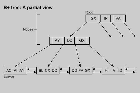
This procedure dictates that the leaf pages become doubly linked lists, allowing their traversal to either the left or right.
Simultaneously, we need to have copies of all the keys inserted in the tree's leaves.
Keys that are located in node pages will be duplicated in the leaves.
This is the first major distinction of the B+ tree: doubly linked leaves containing all entered keys.
The second distinction comes from realizing that since node keys are duplicated in the leaves, we can strip the record data pointers from the node pages.
This makes the data structure of node pages different from that of the leaves.
By contrast, the B-tree has the same structure for both page types.
Figure 1 shows the B+ tree.
Notice that keys in higher nodes are duplicated in each lower node.
This duplication is necessary to locate the proper leaf containing a sought key.
Searching through the B+ tree begins at the root page.
The keys are read and compared with the search key.
The outcome of the comparison normally leads to the next page node.
There the same key comparison is carried out to select yet another page node.
Eventually the obtained pointer will lead to a leaf page.
A final search in the leaf will determine whether or not the sought key exists.
Thus, every search in a B+ tree is equivalent to the worst case search in a B-tree.
However, this fact is not regarded as a serious drawback.
Some people even praise the consistency of the real time involved in searching!
Listing 1 shows the PPL code for searching in a B+ tree.
The main
Search procedure calls upon
SearchNode and Search Leaf to scan the two different types of key pages.
Growth of a B+ tree and a B-tree are similar.
Initially, there is one empty page.
Keys are added and fill out the page.
When an attempt is made to add a key to a full page, the page keys read in memory and the new key is inserted in the key list so that a perfect sorted order is maintained.
Next, the median key is selected, dividing the list into two halves.
The lower half is written back to the old page, while the upper half is written to a newly created page.
Pointers are used to establish the double link between the leaves.
The median itself is stored as the last item of the original page.
A copy of the median key (without the data record pointer) is stored in a new, higher-level node page.
This makes the B+ tree grow by one level.
The page containing the median key becomes the new root page.
A comparison of the median keys will guide the search toward either leaf page.
This scenario takes place during the early growth stages of the B-tree.
When more keys are added, they are inserted in the leaf pages.
As each leaf page becomes full, it is split into halves and the median key inserted into the last location in the leaf pointing to the parent node page.
If the parent node page becomes full, the same operation is carried out, resulting in two new half-full nodes.
Their median is inserted or used to create a new parent node page.
Deleting from B+ trees is more complex than deleting from a B-tree.
If the key deleted occurs in a leaf page only, then the operation is straightforward.
Otherwise, we have two choices to make regarding the deletion of keys from node pages:
♦ Delete the key from the leaf page only.
Keep the keys in the node pages, but mark their status.
Marking can be done by altering a status flag during the search to locate the key to be deleted.
Decide on a criteria for packing the B+ tree.
♦ Delete all occurrences of the key.
This will involve some major rearranging in the node pages.

Figure 1.
 Now let's turn our attention to the B+ + tree.
Its structure serves lo limit the duplication of
keys and make deleting keys more simple.
The B+ + tree is different from ihe B+ tree in the following respects:
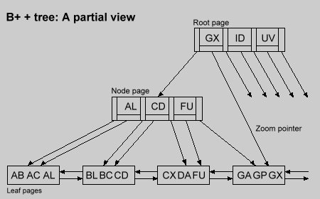
♦ Each key in the node pages has only one duplicate, located in the leaf pages.
♦ The last stored key in each leaf is dedicated to duplicating node keys.
♦ Zoom pointers are attached to each node key.
They point directly to the leaf page containing the key with its record data pointer.
♦ Nodes are doubly linked lists.
♦ Searching in a B+ + tree is not necessarily equivalent to the worst B-tree search.
With a B+ + tree you need one more disk access than with a comparable B-tree search.
When dealing with leaf pages, we declare their capacity.
MAX_KEY, in terms of keys that are not duplicated in nodes.
We deliberately save the (MAX_KEY + 1) position to store the duplicate of a node key.
Each node page is supplied with zoom pointers.
If a search key equals a node key, then it is pointless to continue traversing node pages at lower levels.
The zoom pointer has the address of the leaf page containing full information about the searched key.
The latter is systematically located at the last "hidden" position in the leaf page.
Figure 2 shows the B+ + tree.
B+ + tree and B+ tree searching are similar, with one exception:
once the search key matches a node key, we use the zoom pointer to locate the sought leaf page and recall the last element in the leaf.
Listing 2 shows the PPL code for searching in a B+ + tree.
Growth of the B+ + tree is very similar to that of the B+ tree, with some differences, such as additional zoom pointers in node pages.
Allowing duplicate keys requires establishing double links between all pages.
This is the price to pay for incorporating zoom pointers.
When a leaf page is reached via a zoom pointer, its parent is unknown.
Knowing the parent is not required until the leaf is lull and we need to split the page and insert a copy of the median key into the parent node.
Thus each leaf page must, in turn, know its parent.
A similar argument is used for node pages also.
In case of overflowing keys, each node page must be able to point to its parent.
Deleting a B+ + tree key involves removing it from the leaf pages and any node page that duplicates it.
This requires less node rearrangement than a B+ tree.

Figure 2.
 Since this issue is dedicated to artificial intelligence, a subject of fascination to many of us.
I want to discuss some simple aspects of using statistics in heuristic systems.
During the last decade, much of the programming I've done has revolved around the use of regression analysis in R&D.
The major purpose of this work was to study the correlations between observed variables in an attempt to obtain mathematical models that allow for future predictions.
Attempting to determine the best model is much like detective work.
Statisticians have devised simple and limited methods to select the best models.
Complications arise due to two factors:
applying mathematical transformations to observed data and the varying number of terms in a mathematical regression model.
There is a vast number of combinations for the candidate models.
I will discuss the simplest case for a regression system that learns front experience.
This type of system stores the results of regression calculations and builds a performance history for competing regression models.
Listing 3 shows the PPL code for the system used.
The program is designed to consider a simple linear regression between two variables.
For simplification, only linearized models are considered, each having a slope and intercept, but applying different mathematical transformations.
The system is designed to contain a fixed number of competing models.
This is another simplification.
The coefficient of determination is used to indicate the goodness of fit.
Its values range from zero (meaning no correlation exists) to one (meaning a perfect correlation is obtained).
Every time the program runs, it reads two data files.
The first contains the performance history of the models.
The second contains the observations to be processed.
The program will process the data for each regression model.
All models are used for the first few sets of data, because it is loo early to disqualify any model.
The coefficient of correlation is obtained for each model and is used to update the performance history.
A value close to unity signals good performance.
For the first few sets of data (three in our case) the program stops after all the models are processed.
It is too early to start screening the models.
On the other hand, when enough data sets have been processed, we begin model screening.
We pick the best model, one with the highest average coefficient of determination.
We compare all other models to the selected one.
Using a simple statistical test, we determine, at a certain probability level, whether any other model's coefficient of determination has a statistically different value.
If it does, that model is disqualified and barred from further consideration.
This is done by altering the MAP() identifier.
After this is done, the loop that processes the data will bypass all disqualified models.
This process will continue until a single model is found to fit.
How soon we obtain the model that fits depends on many factors:
♦ The nature of the system studied.
If simple linearized models are not really suitable, then the screening process may take much longer to produce a single, reliable model.
Failing to do so is also meaningful.
It tells us that there is a more complex correlation between the observed variables.
♦ The amount of data in each set processed.
♦ The accuracy of the processed data.
Poor data will throw the system (and any human) off.
These factors reflect a simple heuristic system that learns by storing intermediate results and uses statistical methods to draw conclusions.
Its limitations include the inability to vary the number of terms in the mathematical regression model and to deduce what mathematical transformations should be used.
This area will be discussed in a future column.

PPL code for searching in a B+ tree

---------------------------------------------------------B+ tree

-- DATA TYPE DECLARATION, Pascal style

Leaf_Rec = RECORD
        Leaf_Left, Leaf_Right, Count_Leaf_Key: INTEGER
        Leaf_Key : ARRAY[1..MAX_KEY+1] OF Key_Data
        Leaf_Ptr : ARRAY[1..MAX_KEY+1] OF INTEGER
END RECORD

Node_Rec = RECORD
        Count_Node_Key : INTEGER
        Node_Key : ARRAY[1..MAX_KEY+1] OF Key_Data
        Node_Ptr : ARRAY[1..MAX_KEY+1] OF INTEGER
END RECORD

-- VARIABLE DECLARATION

Leaf : Leaf_Rec
Node : Node_Rec
ROOT, HEIGHT, MAX_KEY, NUM_PAGE : INTEGER


PROCEDURE Search(Soughtkey : Key_Data
                 ROOT, HEIGHT : INTEGER
                 VAR Found : BOOLEAN
                 VAR SoughtLeaf, Sought_Loc : INTEGER
                 VAR Leaf : Leaf_Rec)

-- Search procedure for B+ tree


Found = FALSE
IF HEIGHT > 0 THEN
    INITIALIZE: None
    LOOP
    -- loop will conduct gradual descent in B+ tree
    BEGIN IF HEIGHT <= 1 THEN EXIT END IF
        READ "B+TREE_Key_File",ROOT,Node
        SearchNode(SoughtKey,Node,Found,Sought_Loc)
        ROOT = Node.Node_Ptr[Sought_Loc]
        HEIGHT -= 1
    END LOOP
    TERMINATE: SoughtLeaf = ROOT
               READ "B+TREE_Key_File",SoughtLeaf,Leaf
               SearchLeaf(SoughtKey,Leaf,Found,Sought_Loc)
END IF
END Search

----------------------------------------------------------------

PROCEDURE SearchNode(SoughtKey : Key_Data;
                     Node : Node_Rec;
                     VAR Found : BOOLEAN;
                     VAR Sought_Loc : INTEGER)

BEGIN

    IF SoughtKey < Node.Node_Key[1]
    THEN
      Found = FALSE
      Sought_Loc = 1

    ELSE
     INTIALIZE: Sought_Loc = Node.Count_Node_Key
     LOOP
     BEGIN IF (SoughtKey >= Node.Node_Key[Sought_Loc]) OR
              (Sought_Loc <= 1) THEN EXIT END IF
           Sought_Loc -= 1
     END LOOP
     TERMINATE: Found = (SoughtKey = Node.Node_Key[Sought_Loc])
    END IF
END SearchNode
|
Listing 1.
|
PPL code for searching in a B++ tree

-------------------------------------------------------B++ tree

-- DATA TYPE DECLARATION, Pascal style

Leaf_Rec = RECORD
        Leaf_Left, Leaf_Right, Count_Leaf_Key, Node_Above : INTEGER
        Leaf_Key : ARRAY[1..MAX_KEY+1] OF Key_Data
        Leaf_Ptr : ARRAY[1..MAX_KEY+1] OF INTEGER
END RECORD

Node_Rec = RECORD
        Count_Node_Key, Parent_Node : INTEGER
        Node_Key : ARRAY[1..MAX_KEY+1] OF Key_Data
        Node_Ptr, ZoomPtr : ARRAY[1..MAX_KEY+1 ] OF INTEGER
END RECORD

-- VARIABLE DECLARATION

Leaf : Leaf_Rec
Node : Node_Rec
ROOT, HEIGHT, MAX_KEY, NUM_PAGE : INTEGER

-------------------------------------------------------------------

PROCEDURE Search(Soughtkey : Key_Data
                 ROOT, HEIGHT : INTEGER
                 VAR Found : BOOLEAN
                 VAR SoughtLeaf, Sought_Loc : INTEGER
                 VAR Leaf : Leaf_Rec)

Found = FALSE
IF HEIGHT > 0 THEN
    INITIALIZE: None
    LOOP
    BEGIN IF HEIGHT <= 1 THEN EXIT END IF
        READ #2,ROOT,Node
        SearchNode(SoughtKey,Node,Found,Sought_Loc)
        IF Found THEN HEIGHT = 1;  ROOT = Node.Zoom_Ptr[Sought_Loc]
                 ELSE HEIGHT -= 1; ROOT = Node.Node_Ptr[Sought_Loc]
    END LOOP
    TERMINATE: SoughtLeaf = ROOT
               READ #2,SoughtLeaf,Leaf
               IF NOT Found THEN SearchLeaf(SoughtKey,Leaf ,Found,Sought_Loc)
                            ELSE Sought_Loc = MAX_KEY + 1
END IF
END Search

-- Procedures SearchNode and SearchLeaf are identical to those used
-- with the B+ tree.
|
Listing 2.
|
PPL code for a heuristic statistical system.

PROGRAM SMART_SYSTEM

-- Program to study the best model to correlate observed
-- variables X and Y.  The models used are of the following
-- general type:

--    f(Y) = intercept + slope g(X)

-- where f(Y) is some function of variable Y.
-- where g(X) is some function of variable X.

-- Performance history file contains the following information
--    MAX_MODEL : the maximum number of models compared
--    Remaining_Models : The number of remaining models
--    MAP(): A string containing MAX_MODEL characters to map the status
--           of each model.  If position i has "Y" then the model is
--           still considered.  Otherwise it is disqualified.
--    Model records composed of the following:
--        Sum_R2 : Sum of the coefficient of determination values
--        Sum_Sqr_R2 : Sum of the squares of the coefficient of
--                     determination values
--        Model_Name : A string containing the model name.

-- N is the number of data sets processed
-- X() and Y() are the arrays for the observations.

BEGIN
    Read performance history file
    IF Remaining_Models = 1 THEN DISPLAY "One model, program stopped"
                                 Halt program
    END IF
    Read observed data file
    N += 1
    INITIALIZE: None
    LOOP <Model>
    BEGIN  For Model = 1 TO MAX_MODEL
        INITIALIZE: Set statistical summations to zero
                    i = 1
        LOOP <Data>
        BEGIN IF (i > Num_Data) OR (MAP(Model) <> "Y")
              THEN EXIT <Data> END IF
          CASE i OF
             WHEN 1 => Xreg = X(i); Yreg = Y(i)     -- Linear model
             WHEN 2 => Xreg = Ln(X(i)); Yreg = Y(i) -- Exponential model
             WHEN 3 => Xreg = X(i); Yreg = Ln(Y(i)) -- Logarithmic model
             WHEN 4 => Xreg = Ln(X(i); Yreg = Ln(Y(i)) -- Power model
          END CASE
          Update summations with values of Xreg and Yreg
          i += 1
        END LOOP <Data>
        TERMINATE: None
        Calculate Slope, intercept and coefficient of determination, R2
        Sum_R2 += R2; Sum_Sqr_R2 += R2 * R2
    END LOOP <Model>

    IF N > 3 THEN
        Best = index of model with highest average R2 value.
        INITIALIZE: Display "Best model is";Model_Name(Best)
                    Table_T = "Tabulated" Student-t value calculated
                               at (N-2) degrees of freedom and
                               selected probability level.
        LOOP <Compare>
        BEGIN For Model = 1 to MAX_MODEL
            IF (Model <> Best) AND (MAP(Model) = "Y") THEN
                -- Calculate Student-t statistics
                Term1 = Sqrt(2/N)
                Term2 = Sqrt((Sum_Sqr_R2(Best) + Sum_Sqr_R2(Model)
                         - Sqr(Sum_R2(Best))/N - Sqr(Sum_R2(Model))/N)
                         / (2 * N - 2))
                CalcT = (Sum_R2(Best) - Sum_R2(Model))/(N * Term1 * Term2)
                IF ABS(CalcT) > Table_T THEN MAP(Model) = "N"
                                        Remaining_Models -= 1
                END IF
            END IF
        END LOOP <Compare>
        TERMINATE: Display all models still in competition
    END IF
END SMART_SYSTEM
|
Listing 3.
|
HTML-Bearbeitung von
Werner Cirsovius
Januar 2015
© CL Publications
 In last month's column, we began a discussion on searching techniques that employ tree structures.
We indicated that binary trees were suitable for memory-based searches.
We also introduced the B-tree structure, which is used to perform a disk-based search.
We ended our discussion by pointing out that B-tree searching has its shortcomings.
While searching for single keys is still efficient, it is somewhat clumsy to read a number of keys in sequence.

 Now let's turn our attention to the B+ + tree.
Its structure serves lo limit the duplication of
keys and make deleting keys more simple.
The B+ + tree is different from ihe B+ tree in the following respects:

 Since this issue is dedicated to artificial intelligence, a subject of fascination to many of us.
I want to discuss some simple aspects of using statistics in heuristic systems.